Download: Learning Aim C

C1 – Handling data within a program:

Defining and declaring constants & variables:

• Alphanumeric strings: This is the description of data that is both letter and numbers. For example, ‘5b6f1y’ is a string of alphanumeric characters. These can be used to help explain the availability of text that can be entered or used in a field. For example, an alphanumeric password field.
• Array: This is a fixed series of memory locations. Each location can store a value or be empty. The computer can access any of the locations in a single operation. The size of the array does not change.
• Boolean: This type of variable can only have two possible values, which are True or False.
• Floating point (real): These are decimal numbers.
• Integers: These are whole numbers.
• Objects: This is a universal variable that can store any kinda of data.
• Record: A record variable is a composite variable whose internal components, called fields, can have different data types.
• Strings: This is a variable that can store zero or more characters such as letters, numbers, spaces etc. You cannot use numeric functions such as addition on strings.

Managing Variables:

Parameters can be passed through subroutines in two ways:

• By Value| A copy of the variable will be passed into the subroutine. Changing this copy will not affect the original variable in the main program. This is an example of a local variable. However, if the copied variable has been changed when passed through the subroutine and you want to use it in the main program. You will need to return it.
• By Reference. | The original variable will be passed into the subroutine. The means that the ‘address’ of the variable is passed through the subroutine. This means any changes that occur to the variable in the subroutine will be affected in the main program. This is an example of a global variable.

C2 – Operations:

Relational Operators:

• > Greater than
• < Less than
• >= Greater than or equal
• <= Less than or equal
• == Equal
• != Equal

Arithmetic Operators:

• + Addition
• – Subtraction
• * Multiplication
• // Division (DIV)
• % Modulus (MOD)

C3 – Built-in Functions:

Arithmetic Functions:

• Random() – Generates a random number
• Range() – Creates an array of elements using the range of values in the brackets
• Round() – Rounds a number up or down to the nearest whole number.
• Truncation() r- Rounds a number down to the number of decimal places in the brackets.

String Handling Functions:

String Conversion:

Converting to numeric allows code to use numbers stored as strings in calculations.

• CInt() – Converts to integer
• CDBb() – Converts to float
• CStr() – Converts to string

Manipulating Strings:

• Concatenation: This is joining together to or more string.
• Length: The amount of characters in a string. Can be found through a len() function.
• Position: This is where a character or group of characters are in a string.

General Functions:

• Input(): This lets users enter data into a variable.
• Open(): This connects a program to a data file with an argument defining type of access, for example: read or write.
• Range(): This is a function to return a range object.
• Print(): This sends text to screen or other output such as a data file.

 C4 – Validating Data:

Using validation helps a programmer to ensure that any data entered as input into a program is possible and sensible. Validation applies rules to inputted data. If the data does not follow the rules, it is rejected. This reduces the risk that incorrectly inputted data crashes a program.

Types of Validation:

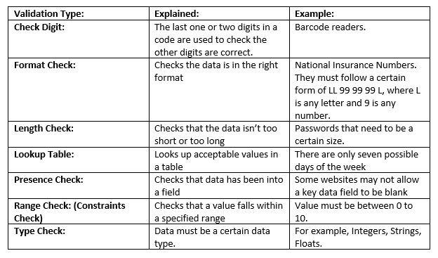
Data Sanitisation:

The purpose of data sanitisation is to hide or protect data so it cannot be seen or disclosed to unwanted users. Examples:

• Masking: This hides visible data by replacing it with something else.
• Input Sanitisation: Checks data that is entered and removes anything that be potentially dangerous. This can help prevent an SQL injection attack.

C5 – Control Structures:

Control Structures analyses variables and choose a direction in which to go based on given parameter. The term ‘control’ details the direction in which the program takes (flows)

There are three types of control structures:

• Sequential: This program follows a default step by step approach. The program is executed line after line.
• Selection: This is used for decisions and to branch to other alternative paths of the program.

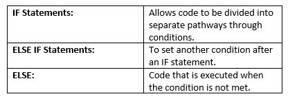
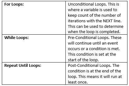
• Repetition: This is used for looping. This repeats multiple pieces of code in a row. Loops can be broken through the BREAK command if no conditional is given.

Modules: (Functions / Procedures)

• Modules are basically created as separate ‘mini programs’. There are blocks of code that sit outside of the main program.
• These modules are then called from the main program when required.
• Modules inspire teamwork. This is because coding each procedure or function can be allocated to different team members depending on their specialties.
• ‘Declaring’ a module means writing the modular code. It is given a name, which is called the header. The body of the module contains instructions, which are a series of code.
• ‘Calling a module’ means naming the module in the main program. The commands stored in the function / procedure are carried out. They carry out in the order you call them. If the module is never called, the code inside the module is never used/executed.
• Good thing about modular programming is that it doesn’t matter what order you make the procedures or what order they are spawn in the code. The sequence of modules is set by the main program. They are carried out in the order they are called.
• Procedures & Functions made by other programmers can be used. This is called a ‘code library’. There are imported into your program. After you import the code library (another word is module), then you can use all the stored procedures/functions in your code.

Advantages of Modular Programming:

• Breaks a large and complex program down into small & manageable parts.
• It allows you to save a block of code, which can be used again and again. This includes being used in future programs.
• It makes programs shorter as it can get rid of repeated code.
• They can make a program more readable depending on the module’s name.
• Work can be allocated between team members.
• It causes less risk of the program breaking / not working as your program can use tried & tested procedures & functions.
• It allows programmers to share their modules via importing procedures / functions made by other programmers.

C6 – Data Structures:

Linked Lists:

A linked list is a dynamic data structure, which is used to store an ordered sequence, as described below:

• The items which form the sequence are not necessarily in contiguous(next or together in sequence) data locations, or in the order in which they occur in the sequence (chronological).
• A linked list can provide a foundation upon which other data structures can be built such as a stacks, queues, graphs & trees.
• A linked list is constructed from nodes & pointers:

1. Each node stores two values. It contains a ‘data field’ and a ‘next address field’.
2. The ‘data field’ holds the actual data associatedwith the list item.
3. The ‘next address field’ contains the address of the next itemin the sequence. This is often known as a pointer. This is always an integer.
4. The ‘next address field’ can also been known as the ‘link’. This is shown by a ‘null pointer’. This means that there are no further items in the list.

 The Array:

• An array is a fixed series of memory locations. Each location can store a value or be empty.
• The computer can access any of the locations in a single operation. The size of the array does not change.

Array Operations:

• Set up an empty array of n
• Add a value to any of the empty slots.
• If you know the index number of an element, you can access it in a single operation.
• If you don’t know the index number of the value you are looking for, you will have to search the array. You can traverse the entire array with a ‘for loop.

One-Dimensional Array:

• It has a single subscript inside the brackets and can be thought as a single list of items. (array[0])
• Can only store one type of data. But can but any type of data. E.g strings or integers

Two-Dimensional Array:

• It is multi-dimensional as it has two subscripts inside the brackets (array[0,0])
• It is a ‘array of arrays’ and can have similar data types instead of being limited to one.

Records:

• Used to store items such as a product or a person, often in a database table.
• Made from fields, each which is defined to an appropriate data type.
• A database query, also known as an Entity Relationship Diagram (ERD), can join tables together into a dataset, which consists of any mix of the table fields and can contain records selected by criteria to be used by forms and reports.

Sets:

• A set consists of some data that has been brought in from a structure such as a table in a database, an array in a program or records that match a criterion.
• Each set will meet a particular requirement.
• A database uses queries to produce data sets, a data set is often temporary and used for a purpose such as providing the data for a report.

C7 – Common Stand Algorithms:

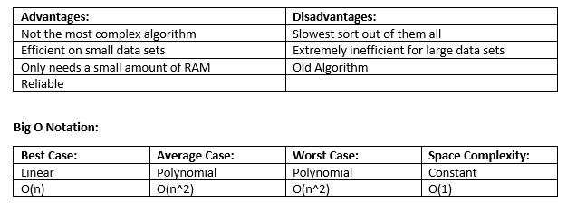
Big-O Notation: is used to express the time complexity, or performance of an algorithm.

• Some algorithms are slower than others. The speed of an algorithm is usually expressed as a function of ‘n’.
• N = the number of items that have to be processed.
• There are three types of speed varies in algorithm:
• Best Case Scenario. (If you were searching for an item in a list and the first term was your search term)
• Average Time.
• Worst Case Scenario (If the search term was the very last term in the list)
• The Big-O represents the increase in processing time as the size of n increases. It is a rating system for the complexity of an algorithm. The higher the ‘Big-O’, the slower the algorithm.
• Best to Worst Times:

1. O(1) – Constant Time. O(1) describes an algorithm that takes constant time (the same amount of time) to execute regardless of the size of the input data set. This is the fastest and least complex.
2. O(log n) – Logarithmic Time. This will grow very slowly as the size of the data set increases.
3. O(n) – Linear Time. This describes an algorithm whose performance will grow in linear time, in direct proportion to the size of the data set.
4. O(n^2) – Polynomial Time. This describes an algorithm whose performance is directly proportional to the square of the size of the data set. A program with two nested loops each performed n times will typically have an order of time complexity O(n^2). The running time of the algorithm grows in polynomial time.
5. O(X^n) – Exponential Time. The number of operations shoots up very high as n increases. This is the slowest and most complex.

Bubble Sort:

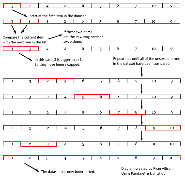
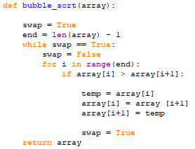
This orders an unordered list of items by comparing each item with the next one and swapping them if they are out of order. The algorithm is finished when no swaps are made. It effectively ‘bubbles up’ the largest (or smallest) item to the end of the list.

Simplified Explanation:  

1. Start at the first item in the list
2. Compare the current item with the next one
3. If the two items are in the wrong position, swap them.
4. Move to the next item in the list.
5. Repeat from step 2 until all the unsorted items have been compared.

 

The Quicksort:

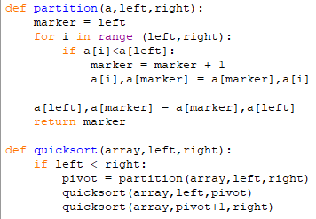
The Quick Sort Algorithm uses a divide & conquer algorithm to quickly reduce the size of a problem.

1. Choose one item to be the ‘pivot’ value. This can be either the first or last value in a data set.
2. Compare every item with the pivot.
3. Divide the list into two ‘partitions’. These are items that are either bigger or smaller than the pivot.
4. Continue recursively until each partition has one item.

Visualised:

9

5

4

15

3

8

11

 

In the unsorted data set above, we have chosen the first value to be our pivot. This is 9. We will now compare 9 with all other values in the data set and divide them into two partitions.

For example: 9 is bigger than 5. 5 is smaller then 9, so it will go into the partition that is smaller than 9. However, 15 is bigger than 9. 15 will go into the second partition that is bigger than our pivot value. In short:

• All elements less than the pivot value must be in the first partition.
• All elements greater than the pivot value must be in the second partition.

3

5

4

8

9

15

11

 

3 and 15 are now the pivots in the left and right partitions. We now use recursion to repeat the process until the list is in sequence.

3

5

4

8

9

11

15

 

3

4

5

8

9

11

15

 

The average time complexity is n*log-n while its worse can be n*n.

Insertion Sort:

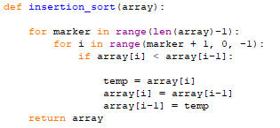
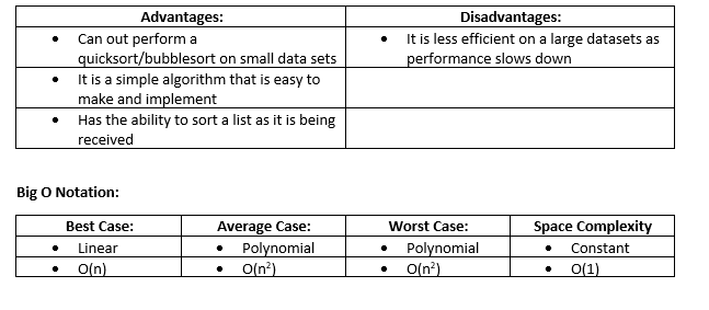
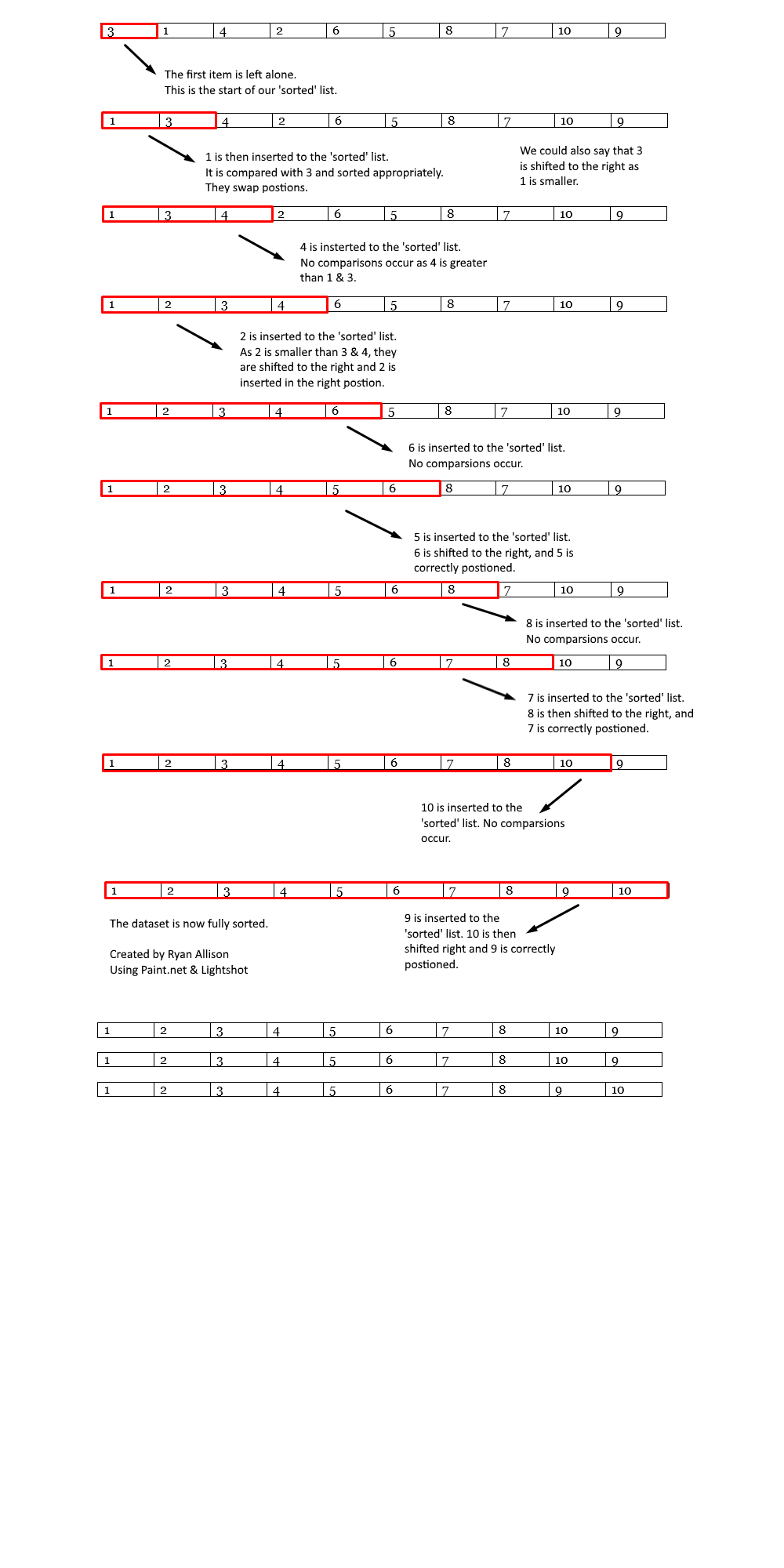
The Insertion sort inserts each item into its correct position in a data set one at a time,

Simplified Explanation:

1. Start at the second item in the list.
2. Compare current item with the first item in the sorted list
3. If the current item is greater than the item in the list, move to the next item in the sorted list.
4. Repeat from step 3 until the position of the current item is less than or equal to the item in the sorted list.
5. Move all the items in the list from the current position up one place to create a space for the current item.
6. Insert the current Item.
7. Repeat from step 2 with the next item in the list until all items have been inserted.

Insertion Sort in Python:

Linear Search:

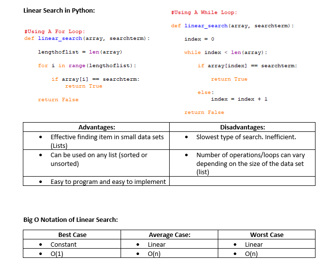
The Linear Search starts at the beginning item in the list and checks each item one by one until it finds the intended search term.

Simplified Explanation:

1. Start at the first item in the list.
2. If this item is the search term, then the search is complete.
3. If the item is not the search term, then move to the next item in the list.
4. Repeat Step 2 until the search term is found or when there are no more items in the list.

Binary Search:

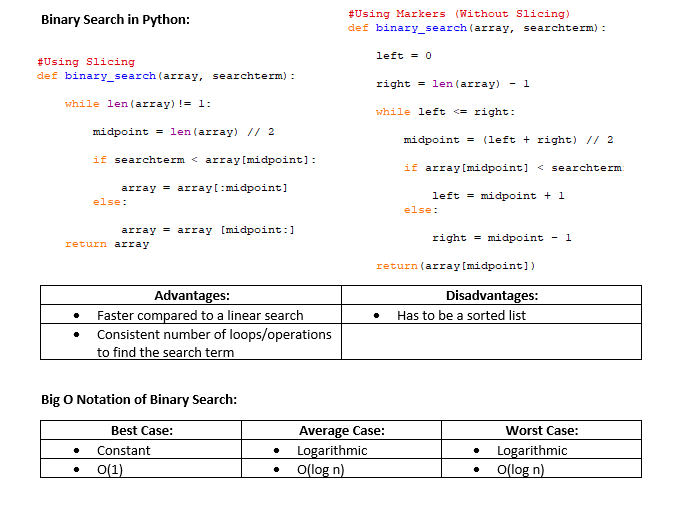
The Binary Search is an efficient algorithm for finding an item in a sorted list. To perform a Binary Search, start at the middle item in the list and repeatedly divide the list in half. (Divide and Conquer approach).

Simplified Explanation:

1. Start at the middle item in the list.
2. If the middle item is the one to be found, the search us complete.
3. If the item to found is lower than the middle item, discard all the items to the right.
4. If the item to be found is higher than the middle item, discard all items to the left.
5. Repeat from step 2 until you have found the item or there are no more items in the list.

Stack:

A Stack is a Last in, First Out (LIFO) data structure. This means that items are added to the top and removed from the top.

Stacks are used in calculations, and to hold return addresses when subroutines are called.

A Stack may be implemented as either a static or dynamic data structure.

5
4
3	D (top of stack)
2	C
1	B
0	A

 

Operations on a stack:

push(item)	Adds a new item to the top of the stack
pop()	Removes and returns the top item from the stack
peek()	Returns the top item from the stack but does not remove it
isEmpty()	Tests to see whether the stack is empty and returns a Boolean value
isFull()	Tests to see whether the stack is full and returns a Boolean value.

 

Advantages of the Stack:

• Data is accessed by a single memory location, which is the top of the stack.
• The Stack makes best use of processor time. Adding or Deleting data is always a single operation O(1). No matter how big the stack is.
• Stack makes the best use of memory space as there no gaps in the data storage.

Disadvantages of the Stack:

• It is an inflexible data structure as you can only access it in one place.
• You can only push & pop.
• You cannot search or sort.
• The computer can’t insert, edit or delete data anywhere but in one place, which is the top.
• The computer cannot traverse this data structure.

The Queue

The Queue is a First In, First Out (FIFO) data structure. This is because the first item you put into the queue will be the first item you will take out. This is useful for when you want to go through data in time order.

• New elements may only be added to the end of a queue. This is called ‘enQueue‘
• Elements may only be retrieved from the front of a queue. This is called deQueue’

Operations On a Queue:

• enQueue(item) – Adds a new item to the end of the queue
• deQueue() – Removes the front item of the queue and returns it
• isEmpty() – Checks if the queue is empty
• isFull() – Checks if the queue is full

Visualising the Queue:

0	1	2	3	4	5	6
“A”

 

We will now enQueue “B”, “C” & “D”

0	1	2	3	4	5	6
“A”	“B”	“C”	“D”

 

We will now deQueue

0	1	2	3	4	5	6
	“B”	“C”	“D”

 

Advantages:

• Data is accessed by two memory locations. The front and the end of the queue.
• It can be used for tasks for when the Stack is not a suitable data structure.
• It makes good use of memory space as there are no gaps.
• It makes good use of processer time as adding or deleting date is just a single operation.

Disadvantages:

• It is an inflexible data structure.
• The locations of the front and end of the Queue are always changing.

 How data is stored in the Queue:

The computer uses pointers to store the start and the end of the queue. This is called the head and the tail.

All the data items stay in the same place. It is only the pointers that move.

For example:

Here are some values stored within a Queue data structure:

0	1	2	3	4	5	6	7	8
“A”	“B”	“C”	“D”	“E”	“F”	“G”

 

We will deQueue

0	1	2	3	4	5	6	7	8
	“B”	“C”	“D”	“E”	“F”	“G”

 

The position where the value “B” is located, is now the start of the queue and “G” is the end of the queue.